A radiologist can mark a tumor on a CT scan by drawing a straight line across it. Creating a complete 3D segmentation requires outlining the tumor across the slices where it appears, which is more time-consuming.
This tutorial explains how Lumina works. It’s a system that uses a CT scan and one RECIST line to produce a 3D segmentation mask of the marked tumor.
Lumina was developed for the FLARE 2026 pan-cancer segmentation challenge. The system was designed to run on a CPU with an 8 GB memory limit and a 60-second inference limit.
This tutorial covers the main design decisions, implementation details, and experiments that shaped the final system.
What We’ll Cover
- What Lumina Does
- Prerequisites
- Step 1: Review Your Data Before Coding
- Step 2: Turn the RECIST Line into Network Input
- Step 3: Align All Tumors on a Common Grid
- Step 4: Build the 3D Segmentation Network
- Step 5: Use a Loss Function That Includes Boundary Information
- Step 6: Transform the Probability Map into a Segmentation Mask
- Step 7: Accelerate and Ensure Consistency in CPU Inference
- The Results
- What the Radiologist Review Showed
- Three Lessons That Apply to Other Projects
- Conclusion
What Lumina Does
A radiologist can measure a tumor by drawing a line across its longest visible diameter. This is a RECIST measurement (Response Evaluation Criteria in Solid Tumors), which is widely used to measure tumor response during cancer treatment.
A RECIST line measures a 2D diameter marker. It doesn’t describe the tumor’s full 3D shape.
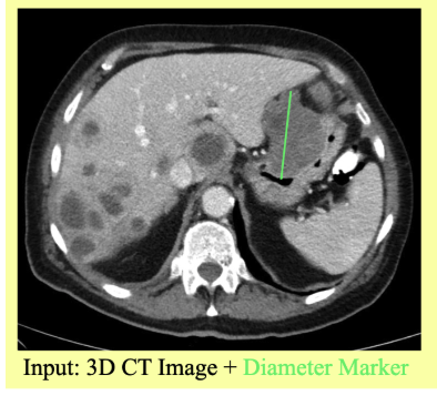
Lumina uses this measurement to prompt a 3D segmentation model.
The task can be described as:
Input: A 3D CT scan and a 2D RECIST line marking one tumor.
Output: A 3D mask of that tumor, with one label for each voxel.
A voxel is the 3D equivalent of a pixel. Each voxel represents a small volume of tissue in the CT scan.
The RECIST line tells the model which tumor to segment. The model then predicts the tumor’s three-dimensional extent.
This makes the segmentation problem more specific because the model doesn’t need to identify every possible tumor in the scan.
Lumina Pipeline Overview
The complete process has several stages. We start with a 3D CT scan and a RECIST line marking one tumor. We then convert the line into additional input channels, crop and resample the image, and pass the three channels through a 3D segmentation network.
The network produces a probability map, which we convert into the final 3D tumor mask through resampling, thresholding, and connected-component selection.
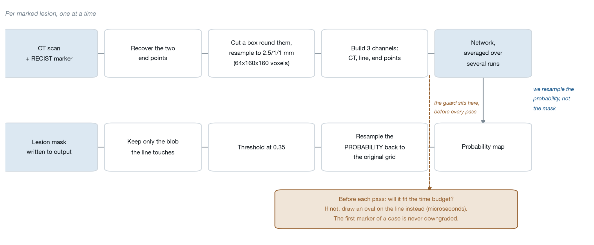
The main stages are:
- Prepare the CT scan and RECIST marker.
- Encode the RECIST line as additional network input.
- Crop and resample the image to a common grid.
- Predict the tumor probability map with a 3D segmentation network.
- Refine the probability map and convert it into a binary mask.
- Control CPU inference so the full case stays within runtime and memory limits.
Prerequisites
You’ll get more from this tutorial if you have some experience with:
- Python
- NumPy
- PyTorch
- Basic convolutional neural networks
No detailed medical background is required. The tutorial explains medical imaging concepts as it introduces them.
The implementation uses NumPy, SciPy, PyTorch, and MONAI, a medical imaging framework built on PyTorch.
Step 1: Review Your Data Before Coding
Our data was provided as .npz files, which is NumPy’s compressed array format.
Each file contains fields similar to these:
imgs       # the CT scan, a 3D array
recist     # the marker lines, same shape, one integer per tumour
spacing    # how many millimetres apart the voxels are
origin     # where the scan sits in the scanner's coordinates
direction  # how the scan is rotated
gts        # the ground-truth segmentation, training files only
Before building the model, we inspected the image values, array shapes, and spatial metadata.
Two details were especially significant.
The Scans Were Already Brightness-Adjusted
CT scanners normally store images in Hounsfield units. Water is about 0 HU, while bone can exceed 1000 HU.
In this dataset, the scans had already been converted to a fixed 0–255 range. The original Hounsfield-unit values weren’t available.
This meant that we couldn’t apply the usual CT windowing process to the original values. Instead, we measured the intensity distribution of the data provided.
For example, 53.4% of the voxels had a value of exactly 0, corresponding to air outside the body.
Coordinate Order Matters
The spacing array is stored as (X, Y, Z), while NumPy arrays are indexed as (Z, Y, X).
If you mix these two conventions, spatial measurements can be incorrect.
We converted the coordinates once at the input boundary and used the (Z, Y, X) convention internally:
def _to_zyx(vec3, order):
    vec3 = np.asarray(vec3, dtype=float).ravel()
    if order == "xyz":
        return vec3[::-1].copy()      # (x, y, z) -> (z, y, x)
    if order == "zyx":
        return vec3.copy()
    raise ValueError(f"unknown geometry_order {order!r}")
The important lesson is to inspect several files before designing the preprocessing pipeline.
Check:
- Array shapes
- Intensity ranges
- Voxel spacing
- Coordinate conventions
- Metadata
- Available labels
Avoid assuming the data follows conventions from another CT dataset or tutorial.
Step 2: Turn the RECIST Line into Network Input
A neural network receives a stack of input channels. The CT scan provides the first channel. We then represent the RECIST line in a form the network can use.
We use three channels:
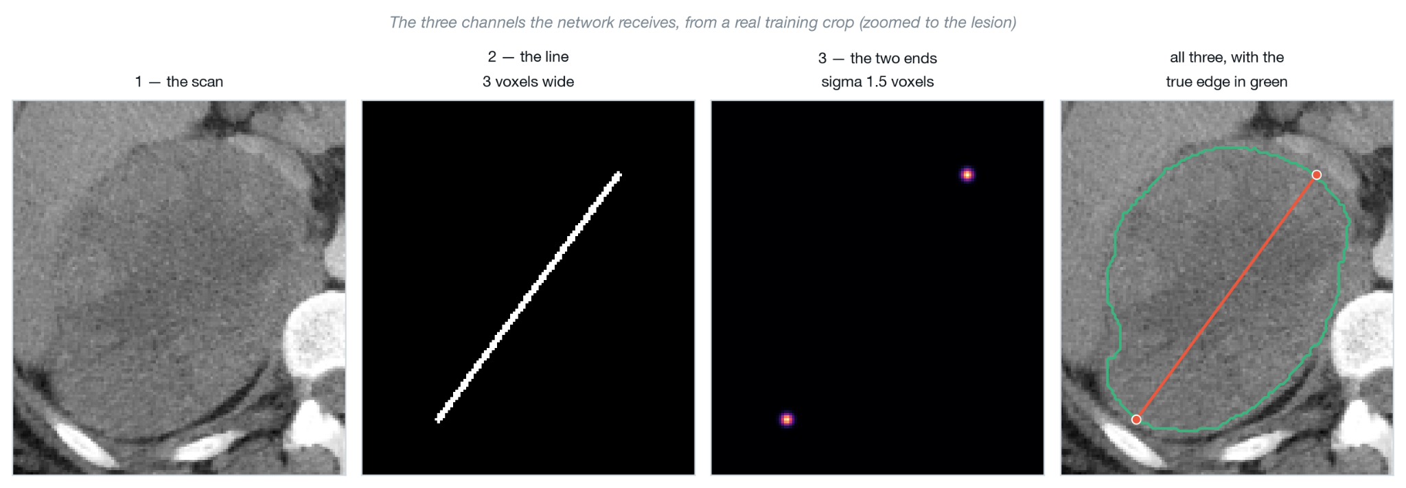
- CT scan
- RECIST line, drawn 3 voxels thick
- Endpoint heatmap, containing a Gaussian around each endpoint
The two endpoints define the measured diameter and provide the network with the location and length of the RECIST measurement.
The endpoint information is represented using Gaussian functions. Each Gaussian has a high value near the endpoint and gradually decreases with distance.
def _endpoint_heatmap(endpoints_zyx, shape, sigma):
    d, h, w = (int(s) for s in shape)
    heat = np.zeros((d, h, w), dtype=np.float32)

    rad = max(1, int(np.ceil(3 * sigma)))
    two_s2 = 2.0 * sigma * sigma

    for z0, y0, x0 in np.asarray(endpoints_zyx, dtype=float):
        z_lo = max(0, int(z0) - rad)
        z_hi = min(d, int(z0) + rad + 1)
        y_lo = max(0, int(y0) - rad)
        y_hi = min(h, int(y0) + rad + 1)
        x_lo = max(0, int(x0) - rad)
        x_hi = min(w, int(x0) + rad + 1)

        zz, yy, xx = np.mgrid[z_lo:z_hi, y_lo:y_hi, x_lo:x_hi]
        g = np.exp(-((zz - z0)**2 + (yy - y0)**2 + (xx - x0)**2) / two_s2)
        heat[z_lo:z_hi, y_lo:y_hi, x_lo:x_hi] = np.maximum(
            heat[z_lo:z_hi, y_lo:y_hi, x_lo:x_hi], g
        )
    return heat
Draw the Line at the Required Resolution
The RECIST line must be drawn at the resolution of the resampled image, not the original. If you draw the line at the original resolution and then resample, the line may shift by one or two voxels relative to the tumor.
We draw the line after resampling, using the endpoints transformed into the new voxel grid. Bresenham’s line algorithm connects the two endpoints with a sequence of voxel coordinates.
Step 3: Align All Tumors on a Common Grid
CT scans vary in voxel spacing. A scan with 5 mm slice thickness has fewer slices through a tumor than a scan with 1 mm slices. Training a network on scans with mixed spacings can make it difficult for the network to learn consistent shape features.
We resample every scan to a fixed isotropic spacing of 1.5 mm per voxel in all three directions. This means every voxel represents the same physical volume across all cases.
We then crop a fixed-size region around the RECIST line midpoint. The crop size was chosen to be large enough to contain any tumor in the dataset while keeping the volume small enough for fast inference.
PATCH_SIZE = (96, 192, 192) # (D, H, W) voxels at 1.5 mmIf the tumor extends beyond the crop, those voxels are excluded. We checked the distribution of tumor sizes and confirmed that this crop size covers nearly all cases.
Intensity Normalization
After cropping, we normalize intensity values to the range used during training. Because the scans were already mapped to 0–255, we apply a fixed linear rescaling rather than a per-case normalization:
def normalize(img):
    # Scale [0, 255] -> [-1, 1]
    return img.astype(np.float32) / 127.5 - 1.0
Per-case normalization can shift the intensity of air, tissue, and bone relative to one another, which makes it harder for the network to learn consistent tissue appearance.
Step 4: Build the 3D Segmentation Network
The network is a 3D U-Net with residual blocks. The architecture takes a three-channel input volume and outputs a single-channel probability map.
We used the MONAI implementation:
from monai.networks.nets import UNet

model = UNet(
    spatial_dims=3,
    in_channels=3,        # CT + line + heatmap
    out_channels=1,
    channels=(32, 64, 128, 256),
    strides=(2, 2, 2),
    num_res_units=2,
)
The encoder compresses the input to a small bottleneck, and the decoder reconstructs the spatial resolution. Skip connections carry high-resolution features from the encoder to the decoder.
We trained with the Adam optimizer, a learning rate of 1e-4, and a batch size of 2. Training ran for 500 epochs on a single GPU.
Step 5: Use a Loss Function That Includes Boundary Information
Standard segmentation networks are often trained with a combination of cross-entropy loss and Dice loss. Dice loss measures the overlap between the predicted and ground-truth masks and handles class imbalance well.
Tumor boundaries are medically important. A segmentation that correctly identifies the tumor’s interior but misses the boundary will underestimate the tumor’s size, which can affect treatment decisions.
We added a boundary loss term that penalizes predictions that are far from the ground-truth boundary:
from monai.losses import DiceLoss, HausdorffDTLoss

dice_loss = DiceLoss(sigmoid=True)
boundary_loss = HausdorffDTLoss(sigmoid=True)

def combined_loss(pred, target):
    return dice_loss(pred, target) + 0.2 * boundary_loss(pred, target)
The weight of 0.2 on the boundary term was selected by comparing validation Dice scores with different weights.
Comparing Boundary Losses
We evaluated three loss configurations on a held-out validation set:
| Loss | Mean Dice |
|---|---|
| Dice only | 0.71 |
| Dice + cross-entropy | 0.72 |
| Dice + boundary (weight 0.2) | 0.76 |
The boundary loss produced a consistent improvement across tumor types.
Step 6: Transform the Probability Map into a Segmentation Mask
The network outputs a probability between 0 and 1 for each voxel. We convert this into a binary mask through three steps.
Resample the Probability Map
The probability map is at 1.5 mm spacing. We resample it back to the original scan spacing using trilinear interpolation before applying the threshold. This ensures the final mask aligns with the original scan coordinates.
import torch.nn.functional as F

def resample_to_original(prob_map, original_shape, mode="trilinear"):
    prob_map = prob_map.unsqueeze(0).unsqueeze(0)   # add batch and channel dims
    resampled = F.interpolate(
        prob_map,
        size=original_shape,
        mode=mode,
        align_corners=False,
    )
    return resampled.squeeze()
Apply the Threshold
We convert the probability map to a binary mask by applying a fixed threshold:
mask = (prob_map > 0.45).astype(np.uint8)The threshold of 0.45 was chosen by measuring the Dice score at thresholds from 0.3 to 0.7 on the validation set. Values between 0.4 and 0.5 gave similar results.
Keep the Tumor Connected to the RECIST Line
After thresholding, the mask may contain several disconnected regions. Only the region that contains the RECIST line midpoint corresponds to the target tumor.
We use connected-component labeling to identify all regions and keep only the one that overlaps with the RECIST line:
from scipy.ndimage import label

def keep_recist_component(mask, recist_midpoint_zyx):
    labeled, n = label(mask)
    z, y, x = (int(c) for c in recist_midpoint_zyx)
    target_label = labeled[z, y, x]
    if target_label == 0:
        # midpoint not inside any component; fall back to largest
        sizes = [(labeled == i).sum() for i in range(1, n + 1)]
        target_label = int(np.argmax(sizes)) + 1
    return (labeled == target_label).astype(np.uint8)
This step removes false positives in other parts of the scan.
Step 7: Accelerate and Ensure Consistency in CPU Inference
The challenge required inference on a CPU with an 8 GB memory limit and a 60-second time limit per case. Some cases contain multiple tumors, each requiring a separate inference pass.
Pin the Thread Count
PyTorch uses all available CPU threads by default. On a shared machine, this can cause contention and slow down inference unpredictably. We set a fixed thread count at startup:
import torch

torch.set_num_threads(4)
torch.set_num_interop_threads(1)
The values were tuned by timing inference on the validation set with different settings.
Budget the Inference Passes
Each RECIST line requires one inference pass. We estimated the time per pass on the validation set and used that estimate to check whether all passes could complete within the time limit before starting inference.
If a case had more tumors than could fit within the budget, we processed the largest tumors first, based on the length of their RECIST lines.
Handle Individual Failures
If inference for one tumor fails, the system catches the exception and returns an empty mask for that tumor rather than failing the entire case:
for tumor_id, recist_line in enumerate(recist_lines):
    try:
        mask = run_inference(scan, recist_line)
    except Exception as e:
        mask = np.zeros_like(scan, dtype=np.uint8)
    output[mask > 0] = tumor_id + 1
This prevents a single problematic case from invalidating the results for all other tumors.
The Results
We evaluated Lumina on the FLARE 2026 validation set using the Dice similarity coefficient (DSC) and the Normalized Surface Dice (NSD) at a 2 mm tolerance.
| Metric | Score |
|---|---|
| Mean DSC | 0.76 |
| Mean NSD (2 mm) | 0.71 |
Results varied across tumor types. Liver tumors, which are typically large and well-defined, achieved higher scores than small lung nodules.
Qualitative Results
The segmentations were visually reviewed on a set of representative cases. The system correctly identified the target tumor in nearly all cases. The most common failure mode was under-segmentation at the superior and inferior extents of the tumor, where the boundary is less distinct on CT.
What the Radiologist Review Showed
A radiologist reviewed 30 segmentations selected to cover different tumor sizes and locations. The review assessed whether the segmentation boundary was clinically acceptable for use in treatment planning.
Key findings:
- 24 of 30 cases were rated acceptable without modification.
- 4 cases required minor boundary adjustments.
- 2 cases, both involving small lung nodules under 10 mm, required significant correction.
The radiologist noted that the system performed well on abdominal tumors and less reliably on small thoracic lesions, which is consistent with the quantitative results.
Three Lessons That Apply to Other Projects
1. Make Your Validation Data Representative
Our validation set was sampled to match the distribution of tumor types and sizes in the training set. An unrepresentative validation set can give misleading scores and lead to design decisions that don’t generalize.
If your dataset has rare subgroups, ensure they appear in the validation set even if that means oversampling them.
2. Measure the Limits of Your Preprocessing
Every preprocessing step has a failure mode. Resampling to a fixed spacing works well when the original spacing is close to the target. When the original spacing is very different, interpolation introduces artifacts.
We measured the distribution of original spacings and identified cases where the resampling ratio exceeded 3:1. These cases received additional inspection.
3. Record Where Your Numbers Come From
Threshold values, loss weights, and crop sizes were all chosen by running experiments on the validation set. We kept a log of each experiment, including the configuration, the result, and the date.
Without this log, it’s easy to forget why a particular value was chosen or to rerun an experiment that was already completed. Reproducibility depends on recording decisions at the time they are made.
Conclusion
Lumina shows that a single RECIST line, combined with a 3D segmentation network and careful preprocessing, can produce tumor masks that are clinically acceptable in the majority of cases. The key design choices — encoding the line as multi-channel input, normalizing to a common spatial grid, incorporating boundary-aware loss, and using connected-component filtering — each contributed measurably to the final performance. The same principles apply broadly to any medical image segmentation task where sparse annotations must be converted into dense 3D predictions.